SST (Small-Sized Telescope)

SST_like configuration with the CHEC-S camera style

import jax
import jax.numpy as jnp
import matplotlib.pyplot as plt

from iactrace import Camera, Telescope, show_image, show_telescope

Load telescope and camera

telescope = Telescope.from_yaml(
    "../../configs/CTAO/SST_like.yaml",
    n_samples=256,
    key=jax.random.key(42),
)
camera = Camera.from_yaml("../../configs/CTAO/CHECS.yaml")

E0804 11:10:35.965717 3122609 numa_hwloc.cc:121] Call to hwloc_set_cpubind() failed: Invalid argument [22]
E0804 11:10:35.965841 3122610 numa_hwloc.cc:121] Call to hwloc_set_cpubind() failed: Invalid argument [22]
E0804 11:10:35.965883 3122611 numa_hwloc.cc:121] Call to hwloc_set_cpubind() failed: Invalid argument [22]

3D scene

scene = show_telescope(telescope, camera=camera)
scene.show(viewer="jupyter")

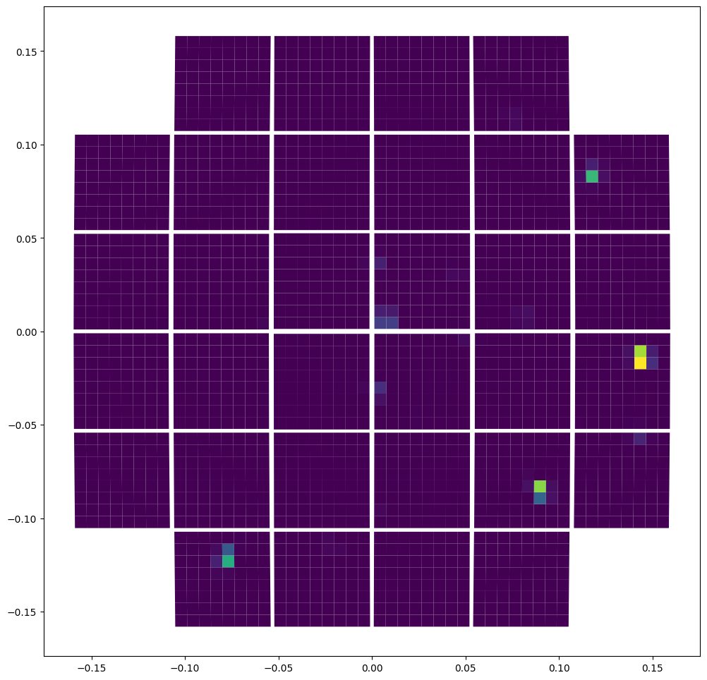
Star field image

n_stars = 100
key1, key2 = jax.random.split(jax.random.key(42))

fov_deg = 7.7
fov_rad = fov_deg * jnp.pi / 180

x = jax.random.uniform(key1, (n_stars,), minval=-fov_rad / 2, maxval=fov_rad / 2)
y = jax.random.uniform(key2, (n_stars,), minval=-fov_rad / 2, maxval=fov_rad / 2)
z = -jnp.ones(n_stars)

stars = jnp.stack([x, y, z], axis=1)
stars = stars / jnp.linalg.norm(stars, axis=1, keepdims=True)

f_stars = 10 ** (-10 * jax.random.uniform(jax.random.key(4242), shape=(len(stars),)))

rays = telescope.render(stars, f_stars, source_type="parallel")
image = camera.image(rays)

fig, ax = plt.subplots(ncols=1, figsize=(12, 12))
ax1 = show_image(image, camera.sensor_groups[0], ax=ax)

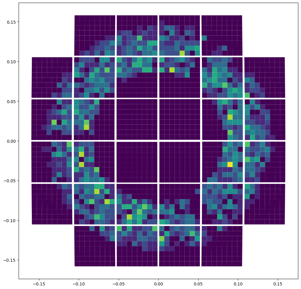
Bokeh from a finite-distance point source

N_points = 1
key1, key2 = jax.random.split(jax.random.key(45))

x = jax.random.uniform(key1, N_points, minval=-0.1, maxval=0.1)
y = jax.random.uniform(key2, N_points, minval=-0.1, maxval=0.1)
z = jnp.ones(N_points) * 30

points = jnp.array([x, y, z]).T
f_points = jnp.ones(len(points))

rays = telescope.render(points, f_points, source_type="point")
image = camera.image(rays)

fig, ax = plt.subplots(ncols=1, figsize=(12, 12))
ax1 = show_image(image, camera.sensor_groups[0], ax=ax)

Spot diagram

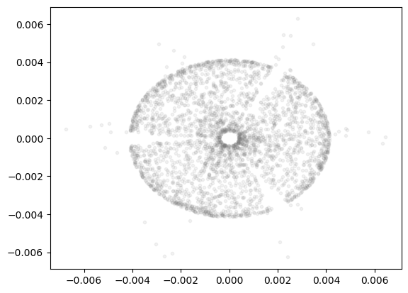
This is created with the focal plane in a position as if the window was non-existent (same as in the optimization). The windows causes a defocus effect of a few mm, which is why the scatter plots looks different.

import jax.numpy as jnp
import matplotlib.pyplot as plt

from iactrace.analysis import AsphericFocalSurface

stars = jnp.array([[0.00, 0.00, -1]])
stars = stars / jnp.linalg.norm(stars)
f_stars = jnp.array([1.0])
rays = telescope.render(stars, f_stars, source_type="parallel")

focal_plane = AsphericFocalSurface(curvature=-1 / 1.06)

hits = focal_plane.intersect(rays)
plt.scatter(
    hits.xy_local[hits.alive, 0], hits.xy_local[hits.alive, 1], alpha=0.1, color="gray", marker="."
)

<matplotlib.collections.PathCollection at 0x14dd9297b080>